I’ve started a project exploring musical instruments and the physics controlling their audio properties. Mostly I’m interested in brass instruments like a trumpet or trombone‒instruments that are tubular for much of their length. Brass instruments have a constant diameter at their beginning. As the tube approaches the end, the instruments become more conical until terminating in a flared bell. I chose them because I played the trumpet in high school. It’s familiar.

One book that I’m using to help understand what is happening is “The Physics of Musical Instruments, 2nd edition” by Neville H. Fletcher and Thomas D. Rossing. It has quantitative descriptions of the properties of real instruments.

One interesting idea is to consider brass instruments as “reed instruments.” For a brass instrument, the “reed” is the lips of the performer. This allows brass instruments to use the same equations as woodwinds. As a first approximation, lips and reeds have similar properties of interrupted air flow. It does make a difference whether the opening closes with increasing pressure or opens with increasing pressure so the analogy has its limits.

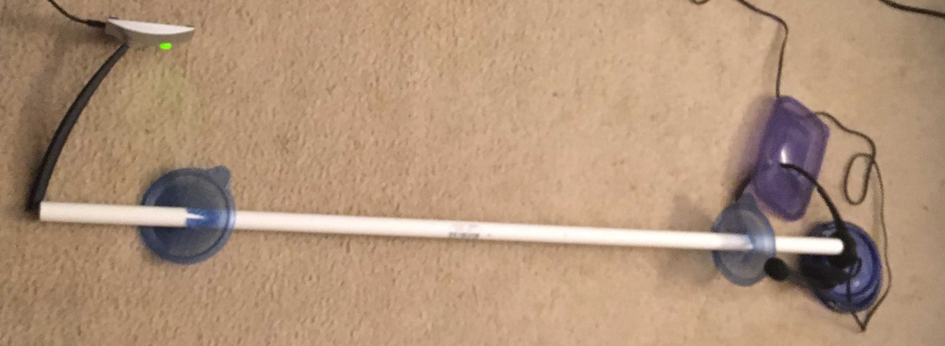
My first experiments have been with a pipe resonating at different frequencies. My method of creating data is to input a sweeping pitched sound to one end of a pipe with a speaker. The pipe resonates at different frequencies so that the intensity of the sound so the other end varies over time. This is a example configuration with headphones presenting the sound on the right end and a microphone picking up sound on the left. I haven’t calibrated the frequency response curve of the microphone and speakers.

For example, when I sweep the input sine wave from 50 Hz to 2000 Hz over 2 minutes on one end of a 1m 1/2″ PVC tube, the amplitude from the other end creates this graph. I measure the amplitude as rms (root mean square) by squaring the values of each sample in a block and then taking their average. This helps in comparing one block to the next.

One thing I notice with such examples is that as the frequency goes up, there is more and more noise in the wave form. The shapes become more ragged. It should be easy to identify the time of the different peaks and thus their frequency but this and other sources of noise interfere.

If I take above run and make an image of its frequency distribution, I get this. The Y axis isn’t calibrated, but starts at 0Hz at the bottom. This chart has the whole duration of a single observation session. The graph above is trimmed to exclude the times that I wasn’t activating the system.

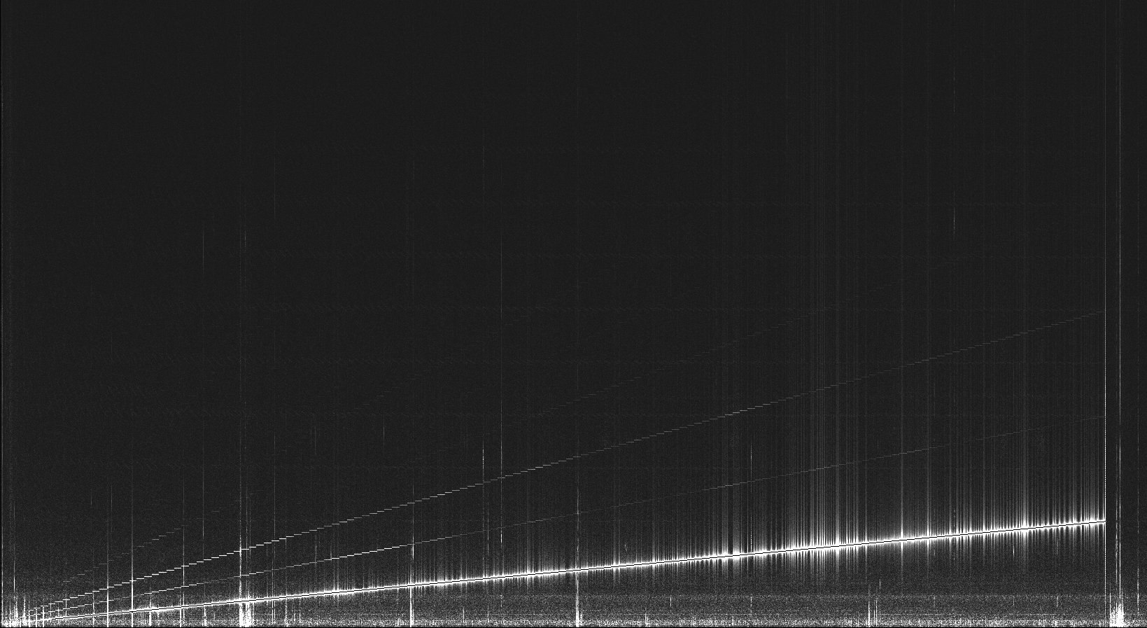
An interesting feature of the graph are the higher overtones from the input sweep. They show up as lines with higher slopes than the main output. This example, I can see 4 extra lines, but different configurations of microphone and pipe may show only one or two. (The third overtone is barely visible above the middle of the run.) Also, if I look closely, I see very faint equispaced horizontal lines. I suspect that those are from my computer fan but I haven’t verified it.

The gray noise at the bottom of the graph are different noises from within my house. I haven’t identified the causes of those or their frequency. Some of the graph is marked with mechanical bumps that show up as lines starting at zero hertz. The vertical features centered on the main input frequency are a common feature of these charts. I’m not sure whether they are real or are an artifact of my processing.

(This representation doesn’t help me identify the position of the peaks.)

An interesting adjustment is needed when I break the signal into chunks. For the Fourier transform or other analyses, I need to block the chunks so that they end at the zero crossings of the input waveform. I pick a minimum number of samples for a block and then search further for the next positively sloped zero crossing. If I don’t do that, the sharp edges at the ends of a block add artifacts that hide real effects. The software I’m using for FFT, FFTW allows me to have non-power-of-two long blocks which is essential for seeing useful results.